
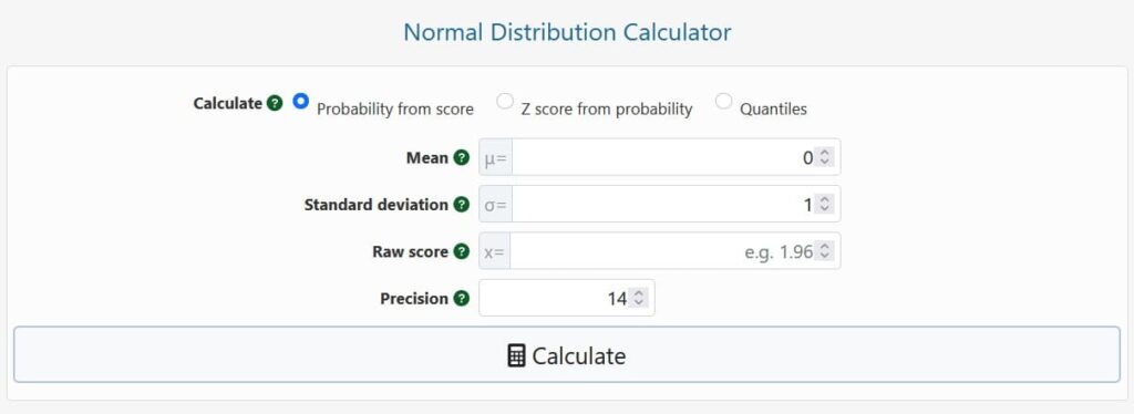
This calculator can be used in three different ways: as a normal CDF calculator, a probability to Z score calculator, or an inverted normal distribution calculator. The first can be used to calculate the chance of an area under a normal curve falling below or above a specified normal score (raw score). A p-value may be computed as part of a statistical significance test, for example. It can also be used to figure out what the significance threshold is for a crucial region defined by one or two standard scores.
The calculations in this mode are performed using the normal distribution’s cumulative distribution function with the supplied mean μ (mu) and standard deviation σ (sigma). The computed Z score is also included in the output. The tool acts as a regular normal distribution calculator with μ = 0 and σ = 1, and the raw score entered equals a Z score.
The inverse CDF of the standard normal distribution is employed in the second mode to compute a standardized score (Z score) matching to the chosen level of statistical significance, also known as the (alpha) threshold. For a one-tailed test of significance, the calculator produces a single z-score (use a minus in front to shift tails if necessary) and two z scores specifying the upper and lower crucial regions for a two-tailed test of significance. These can be utilised in the off-chance that one is required.
The inverse distribution function (IDF) of any normal distribution is computed in quantile mode given the mean, standard deviation, and a certain proportion (a.k.a. quantile). For example, to determine the lower quartile cut-off (lower 25% ) of a normal distribution, simply enter 0.25. Similarly, for the upper decile (top 10% ) cut-off, enter 0.90.
The precision setting specifies how many decimal places the output should be rounded to after the decimal point. It is possible to get a high-accuracy output with up to 25 significant digits.
A continuous probability distribution for a real-valued random variable is the normal distribution (X). Its mean is also its median and mode, and it is symmetrical around the mean. It is commonly referred to as “the Bell Curve” because of its shape, although there are other distributions that produce bell-shaped curves, so this may be misleading. After eminent mathematicians Gauss and Laplace, who were essential in its development and popularization, it is also known as a Gaussian distribution, Gauss, or Gauss-Laplace distribution. The normal distribution’s probability density function yields a graph like the one below.

The normal distribution is non-zero along the whole real line, but on even high-resolution graphs, values above 4 sigma appear to be zero, which is why they are rarely shown.
The fact that the normal distribution can be fully described using only its first two moments (and thus the first two cumulants) – the mean (μ) and the variance (σ2) – is a particularly useful feature. The value of all other moments is zero. Because a distribution’s standard deviation (σ, sigma) is simply the square root of its variance, and because standard deviation is a more useful statistic than variance, a normal distribution is commonly described by its mean and standard deviation.
In the graph above, the standard normal distribution has a mean of 0 and a variance of 1. As a result, its standard deviation is also one. Because the area under the standard normal curve adds up to one, the probability total is one. When the standard deviation is increased, the density of the distribution is distributed more away from the middle point, flattening the form of the distribution. It will become more concentrated around the middle if it is reduced. Normal distributions with any real-valued mean and variance are supported by our calculator.
If a random variable has normally distributed error, critical regions can be established in statistical inference and statistical estimation based on probability values regarded low enough to reject a given hypothesis, as in Null Hypothesis Statistical Testing (NHST). The notion is that if a particular observation is uncommon enough under a specific null hypothesis model, it can be used as evidence against that model and, by proxy, hypothesis. Two critical values are shown in the graph above, at -1.96 and 1.96. On both sides of the distribution, the area they take off adds up to 5% cumulative probability.
The probability density function (PDF) of the normal distribution, the cumulative distribution function (CDF), and its inverse are three fundamental equations for dealing with normally distributed random variables (IDF). The first can be used to get at the second, which can then be used to get a p-value from a z-score. When calculating the z-score from a probability value, the third one is essential.
Probability density function (PDF)
The probability density function of a generic normal distribution with mean and variance 2 has the following formula:

It’s called a “normal distribution formula” for a reason. The density function is used to spread the probability across the distribution’s whole range of possible values (from plus to minus infinity). The rate of change of the normal CDF given below can be represented by the density function.
Standard normal distribution function
These terms can be removed from the previous equation in the case of a standard normal distribution with a mean of zero and a standard deviation of one, simplifying it to:

This formula is also known as the conventional normal distribution formula.
Cumulative distribution function (CDF)
The integral equation for the cumulative probability density function, or cumulative distribution function for short (CDF), of the normal distribution is:

where μ is the mean, σ standard deviation, and x is the z score of interest. The capital Greek letter is commonly used to signify this function Φ (Phi).
Inverse distribution function (quantile function, IDF)
The inverse cumulative distribution function of the normal distribution (a.k.a. ICDF, norm IDF, invnorm, or norminv) is the inverse of the CDF and is given by the equation

where is the mean, and is the standard deviation, and erf-1 is the inverse error function. Normal quantiles are difficult to compute, which is why p value to z score tables were formerly precomputed and distributed. Nowadays, you may quickly determine the inverse function values using a normal distribution probability calculator. Simply pick “Quantiles” from the interface and fill in the blanks.
In the sciences and statistical analyses performed as part of business experiments or observational analysis, the standard normal distribution (μ= 0, σ = 1) is frequently used. Its value lies in generating standardized ratings that may be used to depict statistical discrepancies in a cohesive and easy-to-understand manner. Whether measuring atomic mass displacement, the efficacy of a medical therapy, or changes in consumer behaviors on an e-commerce website, two standard deviations away from the null is two standard deviations away.
Standard scores, often known as Z scores, are quantiles of the standard normal distribution that correspond to particular quantiles. These quantiles are presented for entire z score values below, although they may be calculated for any z score value. Using an inverted normal distribution calculator like ours, calculating a Z score from a chosen p-value threshold is very simple.

It’s crucial to never assume that your data has normally distributed errors or is normally distributed itself while conducting statistical studies. A normality test should be run to see if the normality assumption holds true, but keep in mind that a high p-value from such a test does not always imply that normality can be assumed, especially with small sample sizes. The Central Limit Theorem shows that some useful and extensively used statistics, such as the difference between the means of two distributions of any shape, are regularly distributed (CLT).This makes the normal distribution useful in a wide range of situations where a comparison of distribution means is required.

© 2021 All rights reserved
Ask Your Query