The question is from where did we get these values?
On what basis did market participants come to these values of the premiums?
What are the parameters that affect these values?
Are these fixed by the stock exchanges or by SEBI?
Answer : – Any option’s value increases or decreases depending upon different varia bles. Each variable has its impact on an option.
The impact can be same or different for a call and put option.
Option premium is the sum of intrinsic value and time value.
As long as the option is not expired, there will always be some time value
Intrinsic value may or may not be there, depending upon whether the option is ITM, ATM or OTM.
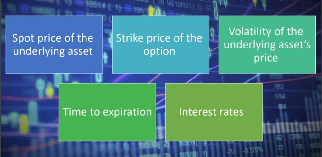
Five fundamental parameters
Spot price of the underlying asset
The option premium is affected by the price movements in the underlying instrument.
If price of the underlying asset goes up the value of the call option increases while the value of the put option decreases.
Similarly if the price of the underlying asset falls, the value of the call option decreases while the value of the put option increases.
Strike Price
If all the other factors remain constant but the strike price of option increases, intrinsic value of the call option will decrease and hence its value will also decrease.
On the other hand, with all the other factors remaining constant, increase in strike price of option increases the intrinsic value of the put option which in turn increases its option value.
Volatility
It is the magnitude of movement in the underlying asset’s price, either up or down.
It affects both call and put options in the same way.
Higher the volatility of the underlying stock, higher the premium because there is a greater possibility that the option will move in‐the‐money during the life of the contract.
Higher volatility = Higher premium, Lower volatility = Lower premium (for both call and put options).
Time to Expiration
The effect of time to expiration on both call and put options is similar to that of volatility on option premiums.
Longer the maturity of the option greater is the uncertainty and hence the higher premiums.
If all other factors affecting an option’s price remain same, the time value portion of an option’s premium will decrease with the passage of time. This is also known as time decay.
Options are known as ‘wasting assets’, due to this property where the time value gradually falls to zero.
Interest Rate
Interest rates are slightly complicated because they affect different options, differently.
For example, interest rates have a greater impact on options with individual stocks and indices compared to options on futures.
To put it in simpler way high interest rates will result in an increase in the value of a call option and a decrease in the value of a put option.
Options Pricing Models
The Binomial Pricing Model
The binomial option pricing model is an options valuation method developed in 1979.
The binomial option pricing model uses an iterative procedure, allowing for the specification of nodes, or points in time, during the time span between the valuation date and the option’s expiration date.
The binomial option pricing model values options using an iterative approach.
With the model, there are two possible outcomes with each iteration—a move up or a move down.
It reduces possibilities of price changes, while removing the possibility for arbitrage.
The model is mathematically simple
Example of Binomial Option Pricing Model
Assume there is a stock that is priced at $100 per share. In one month, the price of this stock will go up by $10 or go down by $10, creating this situation:
Stock price = $100
Stock price in one month (up state) = $110
Stock price in one month (down state) = $90
Next, assume there is a call option available on this stock that expires in one month and has a strike price of $100. In the up state, this call option is worth $10, and in the down state, it is worth $0.
The total investment today is the price of half a share less the price of the option, and the possible payoffs at the end of the month are:
Cost today = $50 – option price
Portfolio value (up state) = $55 – max ($110 – $100, 0) = $45
Given this outcome, assuming no arbitrage opportunities, an investor should earn the risk-free rate over the course of the month. The cost today must be equal to the payoff discounted at the risk-free rate for one month.
The equation to solve is thus:
Option price = $50 – $45 x e ^ (-risk-free rate x T), where e is the mathematical constant 2.7183.
Assuming the risk-free rate is 3% per year, and T equals 0.0833 (one divided by 12), then the price of the call option today is $5.11.
Black Scholes Option Pricing Model
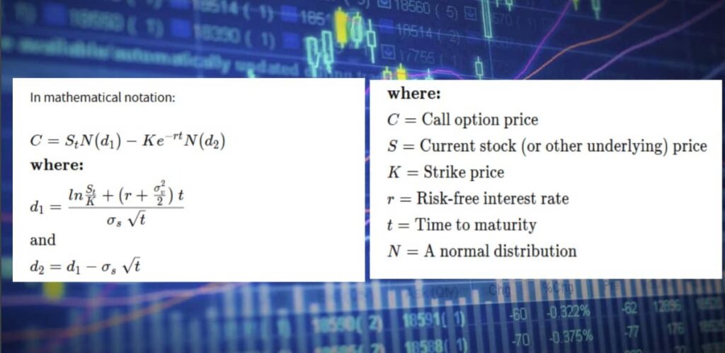
The Black Scholes model, also known as the Black-Scholes-Merton (BSM) model, is a model of price variation over time of financial instruments such as stocks that can, among other things, be used to determine the price of a European call option.
The Black-Scholes Merton (BSM) model is a differential equation used to solve for options prices.
The model won the Nobel prize in economics.
The standard BSM model is only used to price European options and does not take into account that U.S. options could be exercised before the expiration date.
The formula, developed by three economists – Fischer Black, Myron Scholes and Robert Merton – is perhaps the world’s most well-known options pricing model.
Black Scholes Option Pricing Model Assumptions
The Black-Scholes model makes certain assumptions:
The option is European and can only be exercised at expiration.
No dividends are paid out during the life of the option.
Markets are efficient (i.e., market movements cannot be predicted).
There are no transaction costs in buying the option.
The risk-free rate and volatility of the underlying are known and constant.
The returns on the underlying are normally distributed.